
An Introduction to Data Compression
Data compression is a process that makes files smaller, which has the benefit that they take up less space on disk or take less time to transmit over a network. There are many different compression standards such as the zip file format, often used for text files, and MP3 which is used for audio files. Each type of compression is best suited to a particular kind of data. Zip works poorly with audio files and MP3 is unsuited to text files. The correct compression format needs to be applied to the correct type of data.
Some applications would not be possible without data compression. In the early days of the internet it was not feasible to transmit high fidelity audio over a telephone line in real time. The amount of data exceeded the maximum capacity of the line. The MP3 format was originally conceived to deliver acceptable quality audio at the maximum data rate that was achievable via a telephone line at the time.
Transmitting video data over the internet is particularly problematic. An HD video file at 30 frames per second requires about 178 megabytes per second, which is quite a high transmission rate. It is only in recent times that home broadband connections have been offered at all that can achieve this data rate and a mobile phone data contract with a 100 gigabyte allowance would be exhausted in less than 10 minutes. But even where appropriate data capacity is available to the consumer, streaming video service providers would have found it extremely difficult to deliver this data rate to all of their customers simultaneously. Customer expectations are always rising and users now expect resolutions higher than HD. Video compression has enabled the possibility of streaming video via today’s internet technology.
Data compression works by finding a more efficient way to represent the original information. In the following diagram we have a black and white bitmap image of a square on a white background. The image is 8 pixels across and 8 pixels down and is therefore 64 pixels in total. Each pixel is represented by one bit. White pixels are represented by a 0 and black pixels by a 1. The image therefore requires 64 bits in total to store.
Instead of representing the picture as a 2 dimensional grid of pixels, we can put all the pixels in a line like this. It’s the same picture but with the pixels rearranged into a single row instead of an 8x8 grid. The first eight numbers are the top row left-to-right, then the 2nd row left-to-right and so on.
Instead of storing one bit for each pixel, we could instead store a series of counts of how many pixels of each colour there are. Counting from the top left there are 18 white pixels (two rows of 8 and then 2 more = 18 pixels) before we reach a change in colour. Next there are 4x black pixels, then 4x white pixels and so on.
To represent the number 18 in binary we would need 5 bits as 18 = 10010. Then we need to know which colour we are counting, so we could prefix the count with a bit representing the colour. So now we have 010010 to mean count 18x white pixels, that is zero to select white colour followed by 10010 for 18. Next we need to count 4 black pixels so we have 100100 which starts with a 1 to mean select black colour and then the number 4 in binary meaning we should draw 4 pixels in black.
If we use this scheme we end up with this series of bits to represent the entire image:
Now we have only used 54 bits to represent the same picture instead of the original 64 bits. We have compressed the image. Storing the lengths, or runs, of the same colour is called run-length compression.
Run-length compression is one of several forms of lossless compression. The meaning of the term losssless is that we can recover the exact same information that we put in. When we expand out the counts of pixels, an identical image to the one we started with results. In compression though, this is not always the case.
Another form of compression is called lossy compression. This does not recover exactly the same information as was originally put in, but instead produces an approximation of the original information.
In order to reproduce sound, it needs to be represented as a waveform. The chart below is an oscillogram, which is a diagram of an audio waveform:
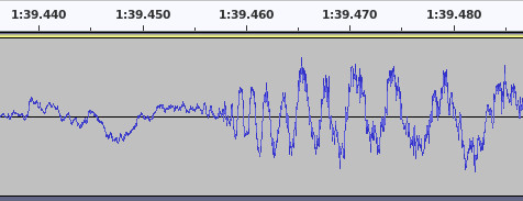
A speaker produces sound by moving a cone backwards and forwards very rapdily using a magnet. The movement of the cone disturbs the air, which your ears are sensitive to. The x-axis of the oscillogram chart represents time. The y-axis represents the position that the speaker cone must move to at that exact instant of time in order to correctly reproduce the intended sound. When the line is near the top of the chart, the speaker cone is fully extended outwards to its maximum forward position and when nearer the bottom the speaker cone is fully withdrawn into the speaker in the opposite direction. When the waveform is at zero, the speaker cone is in the centre position.
Run-length, and most other types of lossless compression, don’t work very well on a waveform as the speaker cone does not stick in one position for very long. The waveform continuously oscillates up and down, therefore there are few continuous runs of the same number to be found in the data and conseqeuently no compression to be had. If you have ever tried to compress a WAV audio file within a ZIP file, you may have noticed it doesn’t make the file particularly smaller. ZIP uses multiple kinds of lossless compression, but none of them work particularly well on audio.
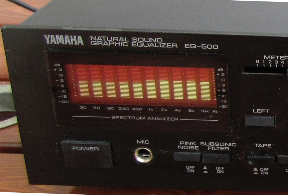
Lossy compression works by transforming the data into a form that is more amenable to standard data compression methods. You may have seen music represented on a spectrum analyser, such as a bar graph that moves in time to the music. These devices are often simulated in music visualisations for streaming audio. The bar chart represents the music as all of the audio frequencies that comprise it at an instant in time. Each bar on the chart is a range of frequencies and the height of the bar represents the loudness of those frequencies. Traditionally, the left-most bar on the graph is a representation of low frequencies and the right-most bar is high frequencies.
If the bar chart is at a fine enough level of detail (if there are enough bars on the chart), it is mathematically possible to convert it backwards from this form into the original waveform the chart was constructed from and therefore actually play the sound that the bar chart represents.
When in this frequency form at a sufficient level of detail, the amount of data needed to store the bar chart is not particularly smaller than the waveform representation that is needed to play the music, however, it has the advantage that we can apply some compression to it.
Sometimes some of the bars are close to zero. This happens when that specific frequency is playing at a very soft volume. If a sound is very soft then the chances are the listener can’t hear it, in which case we can round those specific bars to exactly zero. If we end up with several frequency bars close together that we have rounded down to zero, then we have a run of zeros in the data. In which case run-length compression can be applied and we can compress the audio in bar chart form.
If you imagine the bass drum beat in a song, it is comprised of mainly low frequencies which show up in bars to the left of the chart. During the gaps between each beat of the drum, there may be little else playing in the song that has a low frequency and these bars are close to zero. Therefore we can save on space by avoiding recording the bars representing low frequencies between each drum beat.
Sometimes some of the bars that are not zero are pretty close together (look at the first five bars on the above spectrum analyser). In which case, we can round them to make them exactly the same number. This again means we have a run of identical numbers and can apply run-length compression. Rounding the bars that are similar to be the exact same value is called quantisation.
The problem with rounding out values is that when we reverse the bar chart back into the waveform to play the music, it’s not quite the same as what we originally put in. There are losses, hence it is lossy. People with particularly good hearing might be able to tell the difference, but most people probably can’t. The fidelity of the music depends on the number of bars on the chart and the extent to which we round up and down the values. The more rounding we do, the better the compression because we get longer runs of bars with the same value, but the greater the losses and the greater the chance someone will hear the difference.
There are lossless compression methods that can reduce the size of audio data, such as the FLAC data format, but not to the same extent as lossy methods. The vast majority of audio heard from the internet is lossy compressed.
Lossy compression isn’t any use for storing data where the output needs to be identical to the input. For example you could not use lossy compression for storing software as every byte needs to be correct otherwise the software won’t work. Lossy compression is useful where a person perceiving the data won’t notice the difference, hence it is also sometimes called perceptual compression.
Another compression trick is called temporal compression. This works by looking for regions that are the same between one data item and the one following it. This concept is widely used in video compression. Video is composed of a series of still images or frames. Many video frames do not change a great deal from one frame to the next. Video compression breaks down the image into squares and then checks if any given square has changed on the next frame compared with the current one. If it hasn’t, then the square is stored only once and shared between both frames.
In the below example, showing two frames of video, we mark squares that are the same on both frames. Between the frames the rabbit and the butterfly move, causing the squares covering those characters to be slightly different, however much of the background remains identical. The identical squares for the background only needs to be stored once and can be used for both frames.
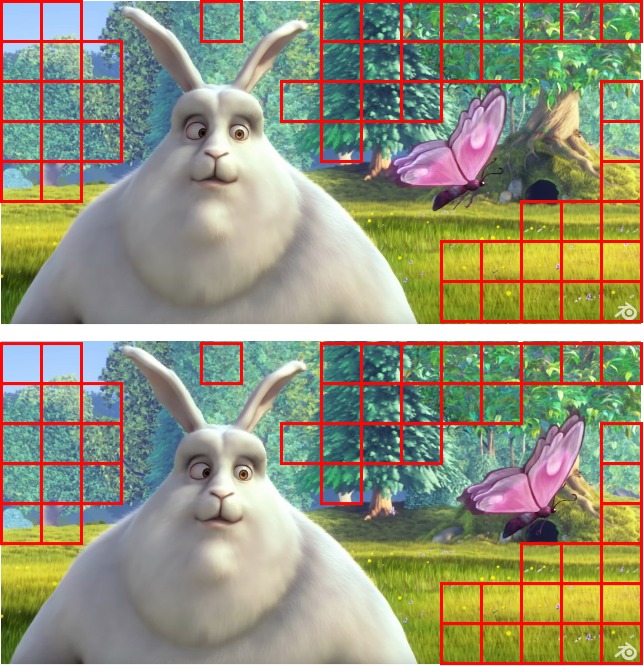
Squares resulting from temporal compression can occasionally be seen in internet video when something goes wrong with the connection. Squares that have changed from a previous frame and should be replaced can incorrectly remain on the screen as the video player has failed to receive anything appropriate to replace them with in sufficient time.
Image Credit: Spectrum Analyser - Touho_T, Big Buck Bunny - Blender